Regression Diagnostics for Linear Models

Provides regression diagnostics for a linear models fit with lm or regress.

# S3 method for lm
diagnostics(x, alpha = 0.4, span = 0.8, plot = TRUE, ...)

Arguments

x: an object of class "lm"
alpha: numeric; transparency for plot points (default=0.4)
span: numeric; smoothing parameter for loess fit lines (default=0.8)
plot: logical; If TRUE (the default), graphs are printed. Otherwise, they are returned invisibly.
...: not currently used

A five component list containing ggplot2 graphs: qqplot, crplots, slplot, vifplot, and influenceplot.

The diagnostics function is a wrapper for several diagnostic plotting functions:

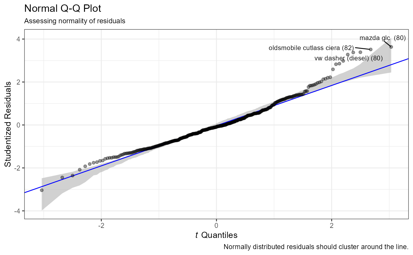
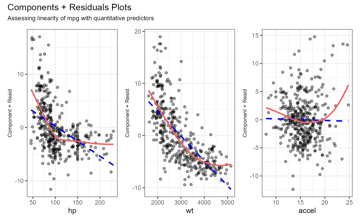
Normality: Normality of the (studentized) residuals is assessed via a Normal Q-Q plot (qq_plot).
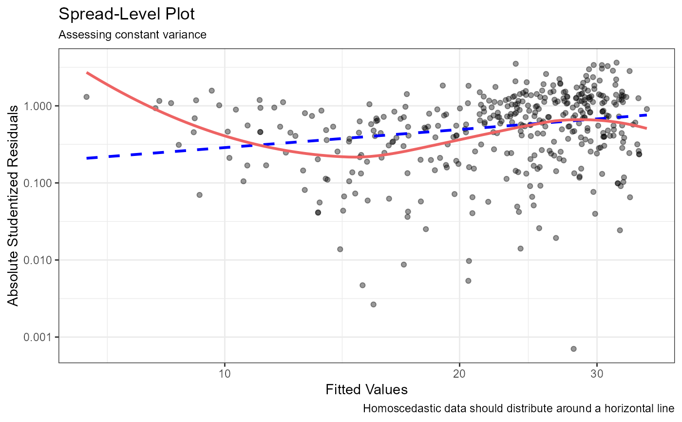
Linearity: Linearity of the explanatory-response relationships are assessed via Component + Residual (partial residual) plots (cr_plots). If there is a single predictor, a scatter plot with linear and loess lines is produced.
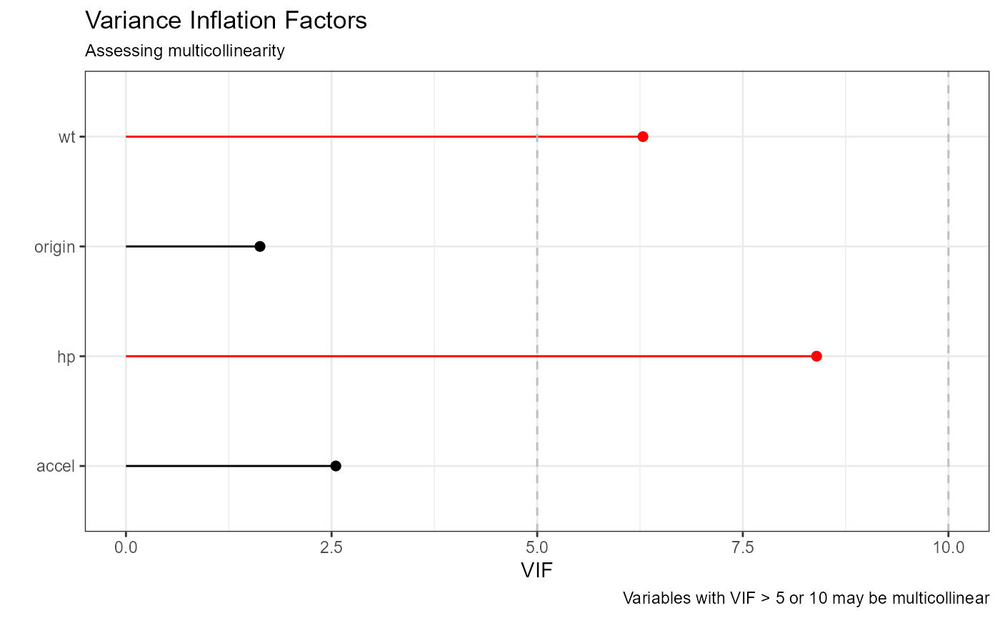
Constant variance: Homoscedasticity is evaluated via a Spread-Level plot (spread_plot).
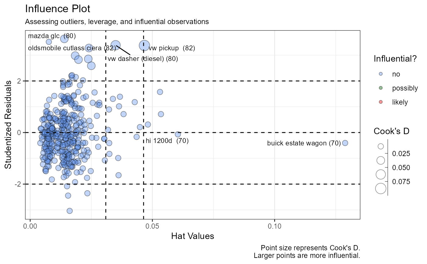
Multicollinearity: Multicollinearity is assessed via variance inflation factors (vif_plot). If there is a single predictor variable, this section is skipped.
Outliers, leverage, and influence: A influence plot identifies outliers and influential observations (influence_plot).

Each function relies heavily on the car package. See the help for individual functions for details.

fit <- lm(mpg ~ hp + wt + accel + origin, data = auto_mpg)
diagnostics(fit)