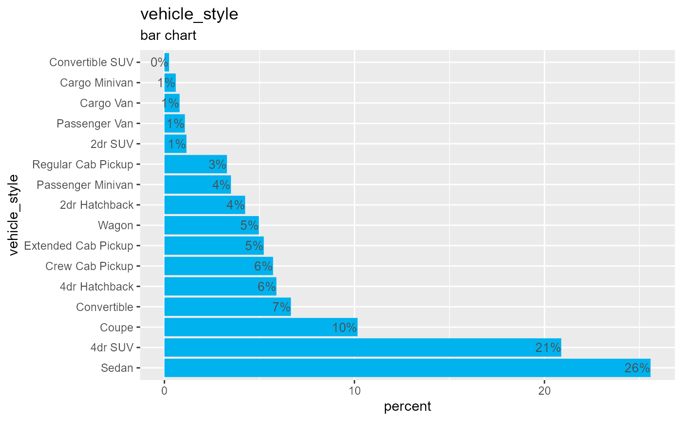
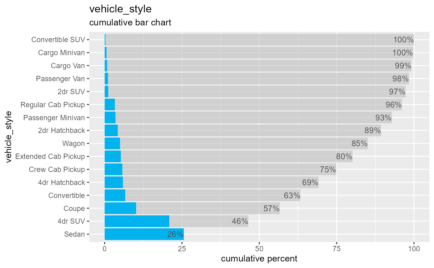
The tab function provides a frequency table for a
categorical variable. Many options are available.
Creating a frequency table
The cardata data frame contains information on 11,914 vehicles, including make, model, and features and price. First, let’s tabulate the number of automobiles by drive type.
tab(cardata, driven_wheels)
#>              level    n percent
#>    all wheel drive 2353  19.75%
#>   four wheel drive 1403  11.78%
#>  front wheel drive 4787  40.18%
#>   rear wheel drive 3371  28.29%
Next, lets add a Total category.
tab(cardata, driven_wheels, total=TRUE)
#>              level     n percent
#>    all wheel drive  2353  19.75%
#>   four wheel drive  1403  11.78%
#>  front wheel drive  4787  40.18%
#>   rear wheel drive  3371  28.29%
#>              Total 11914    100%
Sorting by category
Next, we’ll tabulate the cars by driven_wheels and sort the results in descending order.
tab(cardata, driven_wheels, total=TRUE, sort=TRUE)
#>              level     n percent
#>  front wheel drive  4787  40.18%
#>   rear wheel drive  3371  28.29%
#>    all wheel drive  2353  19.75%
#>   four wheel drive  1403  11.78%
#>              Total 11914    100%
Collapsing categories
Next, let’s tabulate the automobiles by make, sorting from largest number to smallest number. We’ll also remove all missing observations from the data set, add a total row, and limit the makes to the 10 most frequent, plus an “Other” category.
tab(cardata, make, sort = TRUE, na.rm = TRUE, total = TRUE, maxcat=10)
#>       level     n percent
#>   Chevrolet  1123   9.43%
#>        Ford   881   7.39%
#>  Volkswagen   809   6.79%
#>      Toyota   746   6.26%
#>       Dodge   626   5.25%
#>      Nissan   558   4.68%
#>         GMC   515   4.32%
#>       Honda   449   3.77%
#>       Mazda   423   3.55%
#>    Cadillac   397   3.33%
#>       Other  5387  45.22%
#>       Total 11914    100%
Finally, let’s list the makes that have at least 5% of the cars, combining the rest into an “Other” category.
tab(cardata, make,  minp=0.05)
#>       level    n percent
#>   Chevrolet 1123   9.43%
#>       Dodge  626   5.25%
#>        Ford  881   7.39%
#>      Toyota  746   6.26%
#>  Volkswagen  809   6.79%
#>       Other 7729  64.87%
